Get Started
Why DGGS.jl ?
Discrete Global Grid Systems (DGGS) tessellate the surface of the earth with hierarchical cells of equal area, minimizing distortion and loading time of large geospatial datasets, which is crucial in spatial statistics and building Machine Learning models. DGGS native data cubes use coordinate systems other than longitude and latitude to represent the special geometry of the grid needed to reduce the distortions of the individual cells or pixels.
Installation
Currently, we only develop and test this package on Linux machines with the latest stable release of Julia.
Install the latest version from GitHub:
using Pkg
Pkg.add(url="https://github.com/danlooo/DGGS.jl.git")
Convert coordinates
Convert into DGGS zone ids:
using DGGS
lon, lat = (50.92, 11.58)
resolution = 20
cell = to_cell(lon, lat, resolution)Cell{Int64}(186013,262007,3,20)and back:
to_geo(cell)(50.919978678322614, 11.580000174893085)This will return the geographical coordinates of cell center. The higher the resolution, the less will be the discretization error.
Convert data into DGGS
Lets create some data in geographical space:
using DimensionalData
using YAXArrays
lon_range = X(180:-1:-180)
lat_range = Y(90:-1:-90)
geo_data = [exp(cosd(lon)) + 3(lat / 90) for lon in lon_range, lat in lat_range]
geo_array = YAXArray((lon_range, lat_range), geo_data)
┌ 361×181 YAXArray{Float64, 2} ┐
├──────────────────────────────┴─────────────────────────── dims ┐
↓ X Sampled{Int64} 180:-1:-180 ReverseOrdered Regular Points,
→ Y Sampled{Int64} 90:-1:-90 ReverseOrdered Regular Points
├────────────────────────────────────────────── loaded in memory ┤
data size: 510.48 KB
└────────────────────────────────────────────────────────────────┘Plot the geo data:
using GLMakie
plot(geo_array)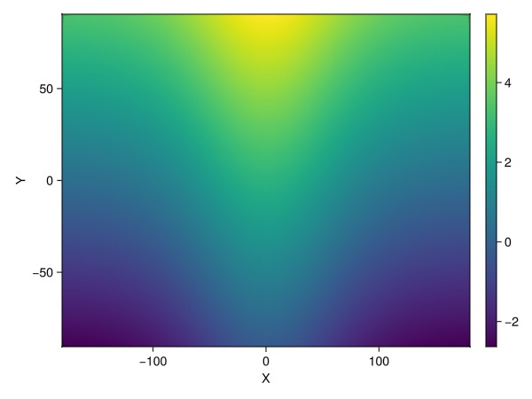
Convert it into DGGS:
resolution = 4
dggs_pyramid = to_dggs_pyramid(geo_array, resolution, "EPSG:4326")
┌ DGGSPyramid ┐
├─── branches ┤
:dggs_s1 dims: dggs_i, dggs_j, dggs_n size: 4×2×5 layers: :layer1
:dggs_s2 dims: dggs_i, dggs_j, dggs_n size: 8×4×5 layers: :layer1
:dggs_s3 dims: dggs_i, dggs_j, dggs_n size: 16×8×5 layers: :layer1
:dggs_s4 dims: dggs_i, dggs_j, dggs_n size: 32×16×5 layers: :layer1
├─────── DGGS ┤
DGGSRS: ISEA4D.Penta
Geo BBox: Extent(X = (-180, 180), Y = (-90, 90))
└─────────────┘Extract a single variable at a given spatial refinement level:
dggs_array = dggs_pyramid[3].layer1┌ 16×8×5 DGGSArray{Union{Missing, Float64}, 3} ┐
├──────────────────────────────────────────────┴───────── dims ┐
↓ dggs_i Sampled{Int64} 0:15 ForwardOrdered Regular Points,
→ dggs_j Sampled{Int64} 0:7 ForwardOrdered Regular Points,
↗ dggs_n Sampled{Int64} 0:4 ForwardOrdered Regular Points
├──────────────────────────────────────────────────────── DGGS ┤
DGGSRS: ISEA4D.Penta
Resolution: 3 (up to 6.40e+02 cells)
Geo BBox: Extent(X = (-180, 180), Y = (-90, 90))
└──────────────────────────────────────────────────────────────┘Plot the array:
plot(dggs_array)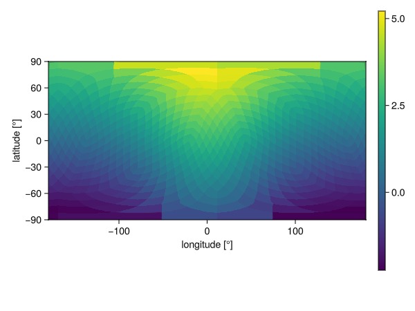
The resolution is set extremely low to demonstrate the cell shapes. In practice, one sets it high enough to prevent losing spatial resolution.